Evaluating Model Performance
Note that the explanations in this section are oversimplified. While we try to capture the intuition behind model outputs and model performance metrics, every object detection algorithm works differently and details differ. If you have any questions, Contact Us!
Interpreting the Graphs
Once model training is in progress, you can click on the relevant model on the training page to view training progress. There, you will see graphs monitoring training progress and model performance.
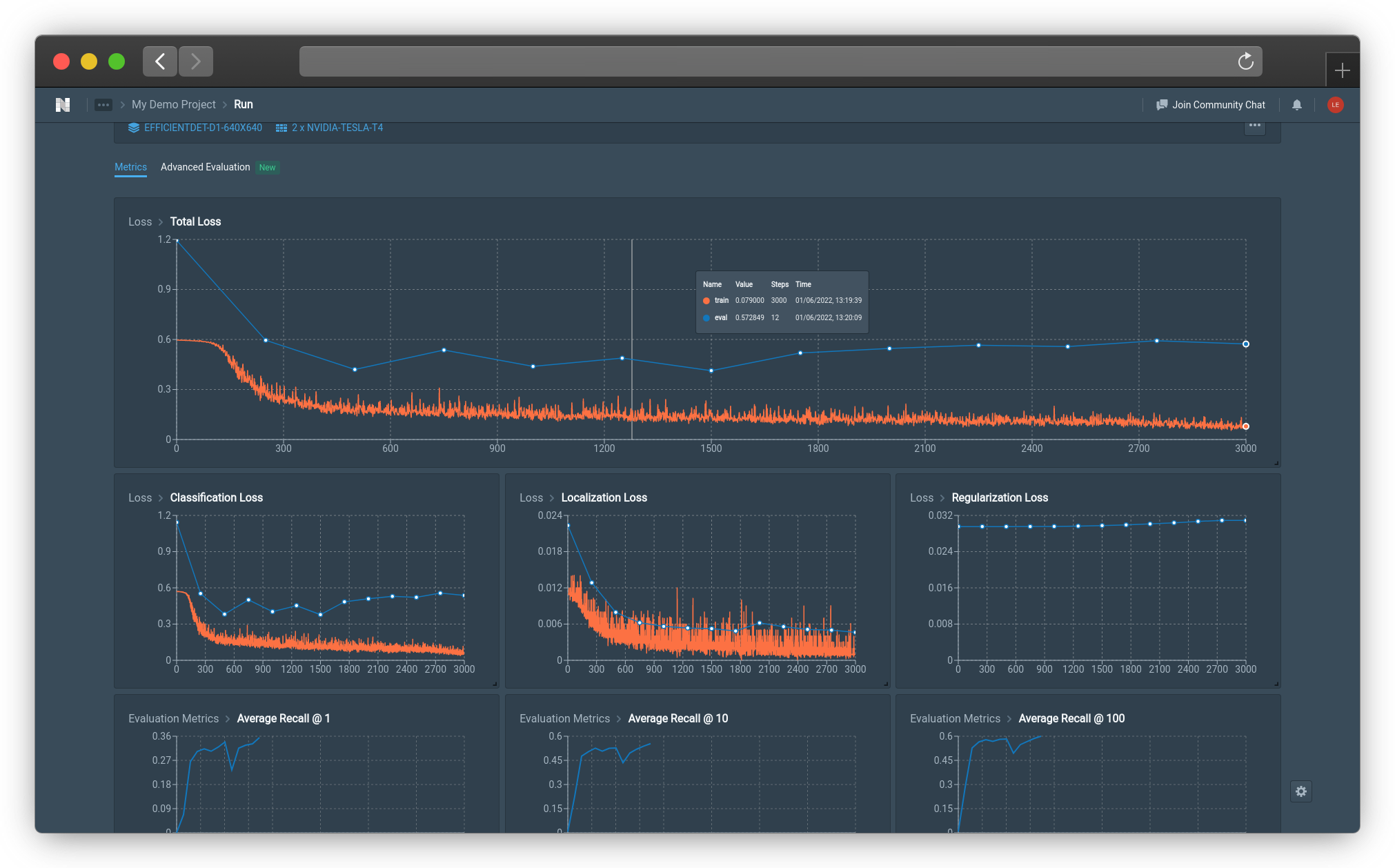
Graph of Classification Loss (Click image to enlarge)
A training step is considered each time model weights are updated, which occurs after every batch of training data is run through the model. Thus, for those more familiar with epochs, the number of training steps can be computed as
Number of Epochs * (Dataset Size/Batch Size) = Number of Steps
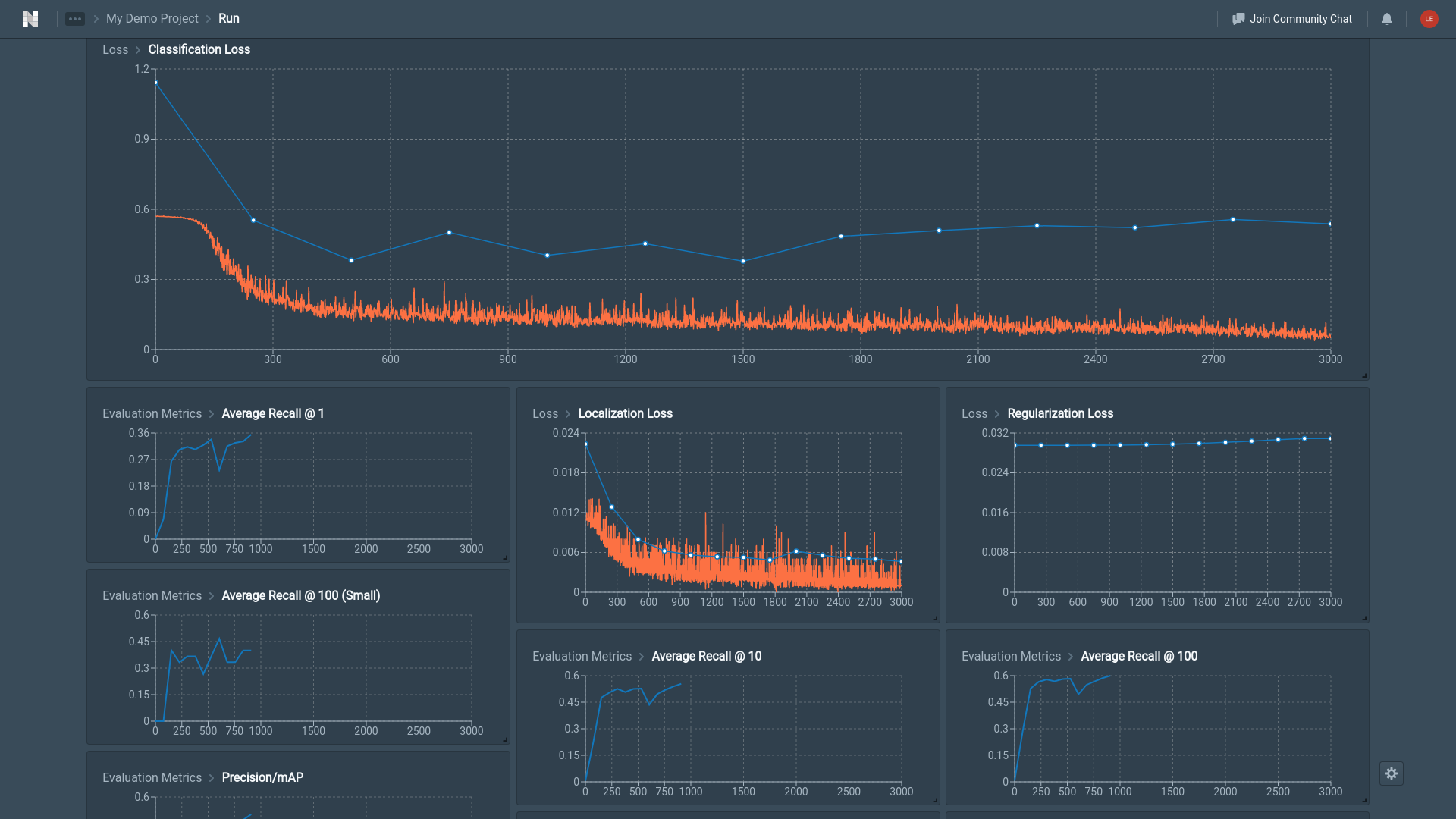
The example above shows a graph of Classification Loss as training progresses. The x-axis represents the number of training steps that the model has trained for, while y-axis represents the loss.
The orange line represents the loss for the training set, and the blue line represents the loss for the test set. This train-test split was selected in the Module : Dataset of the workflow. It splits the model into a train set that will be used to train the model, and a test set used to evaluate the model. Metrics for the train dataset are calculated every epoch, while metrics for the test set are calculated every set number of training steps which can be set during the workflow.
Model Performance Metrics
Metrics used to measure model performance can be categorized as:
Type of Metric | Applicable Model Types |
|---|---|
| |
| |
|
Output of Object Detection Algorithms
To interpret model performance, we need to first understand the output of object detection algorithms.
Given an image, object detection algorithms detect 0 or more objects. Each of these detected objects is denoted by:
- A bounding box indicating the coordinates of the object
- Class of object detected. Only objects present in the training set can be detected
- (Only for Mask RCNN) A per-pixel mask predicting whether each pixel belongs to this object
The model performance metrics for General Loss , Detection Boxes, and Masks are calculated based on how the predicted objects deviate from the respective ground truth objects, based on the discrepancy in bounding box coordinates, object class, and per-pixel masks.
General Loss Metrics
There are 4 general metrics used to measure loss across all models: Total Loss, Classification Loss, Localization Loss,, Regularization Loss.
Comparing Losses
Losses can only be compared across models with the same parent algorithm and the same input size (e.g. RetinaResNet50 640640 vs Retina MobileNetV2 640640).
Losses of models from different parent algorithms (e.g. RetinaNet vs FasterRCNN) cannot be compared, as different algorithms use different formulas for calculating loss.
Losses of models with the same parent algorithm, but with a different input size (e.g. RetinaResNet50 640640 vs RetinaResNet50 10241024) cannot be compared, as several algorithms include the image size when calculating loss.
Total Loss
Total loss is simply the sum of all losses used, so the classification loss, localization loss, and regularization loss.
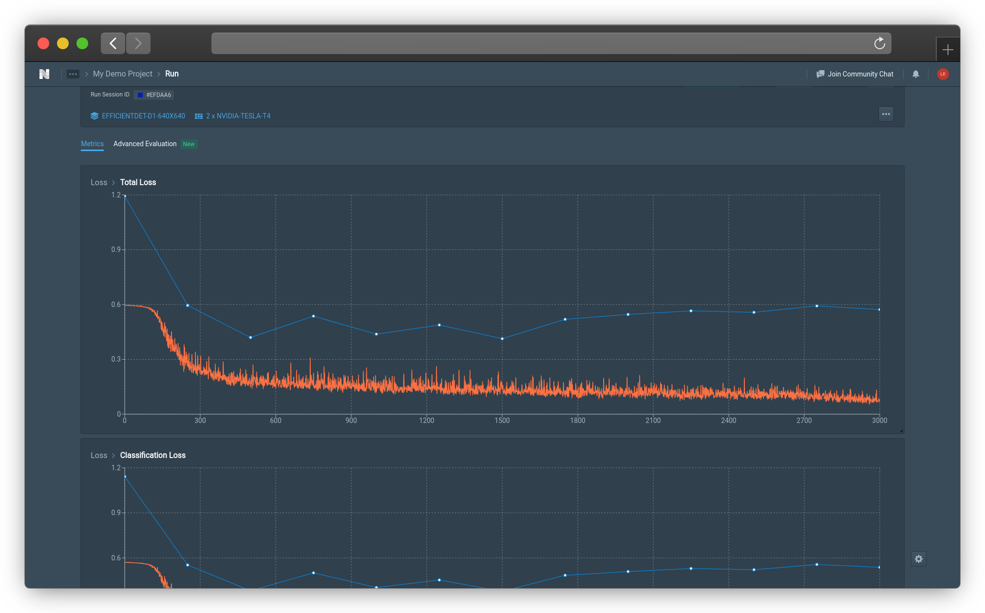
Total Model Loss (Click image to enlarge)
Classification Loss
Classification loss is calculated based on the deviation between the predicted object class of each predicted bounding box, and the ground truth object class in the predicted bounding box.
Generally speaking, if a predicted bounding box has a large overlap with a ground truth bounding box, the predicted class should be the same as the object class of the ground truth bounding box (Assuming there is no other better ground truth overlap).
There might be cases where the predicted bounding box has no significant overlaps with any ground truth bounding box. Different algorithms handle this scenario differently. Some algorithms handle this by setting the ground truth class of such bounding boxes to be "background", meaning the bounding box does not contain any valid objects.
The image below shows an example object detection prediction. There is no classification loss incurred on the Cat prediction, as the ground truth is indeed a cat. There will be a classification loss incurred on the Dog prediction, as it should be predicted as background (depending on the specific algorithm).

Example Object Detection Prediction (Click image to enlarge)
Ideally, the predicted class of objects in predicted bounding boxes should be the same as the ground truth. This will lead to a low classification loss.
Classification loss should reduce on the train set (the orange line) as training progresses.
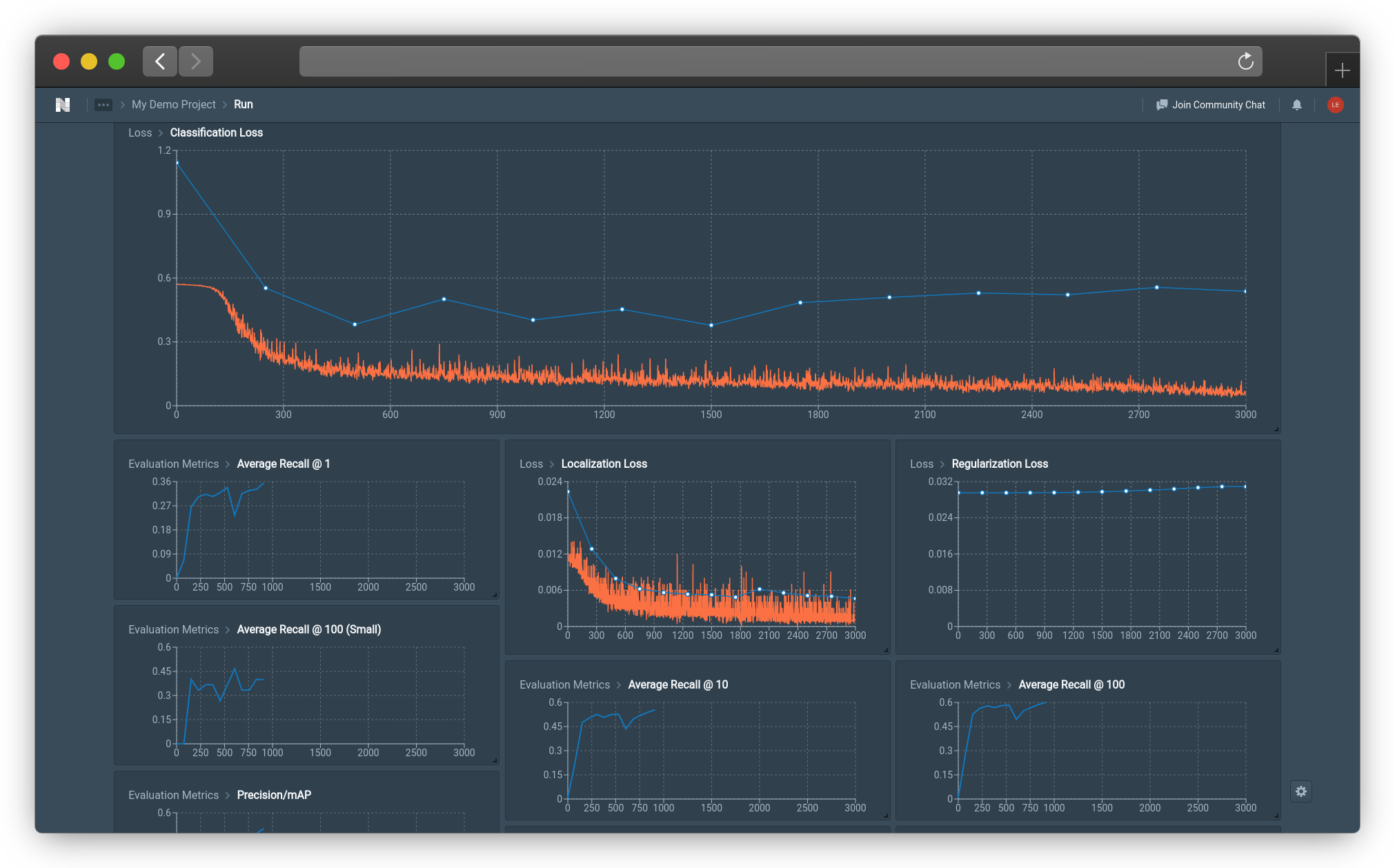
Classification Loss of Model (Click image to enlarge)
Localization Loss
Localization loss is calculated based on the deviation between the coordinates of each predicted bounding box, and the ground truth bounding box.
Generally speaking, each predicted bounding box is mapped to a ground truth bounding box based on the overlap between predicted and ground-truth bounding boxes.
The image below shows an example object detection prediction. There is some localization loss incurred on the Cat prediction, as the predicted bounding box does not capture the ground truth bounding box (the whole cat). In general, there will be no localization loss incurred on the Dog prediction, as the predicted class is wrong (this will depend on the specific algorithm).
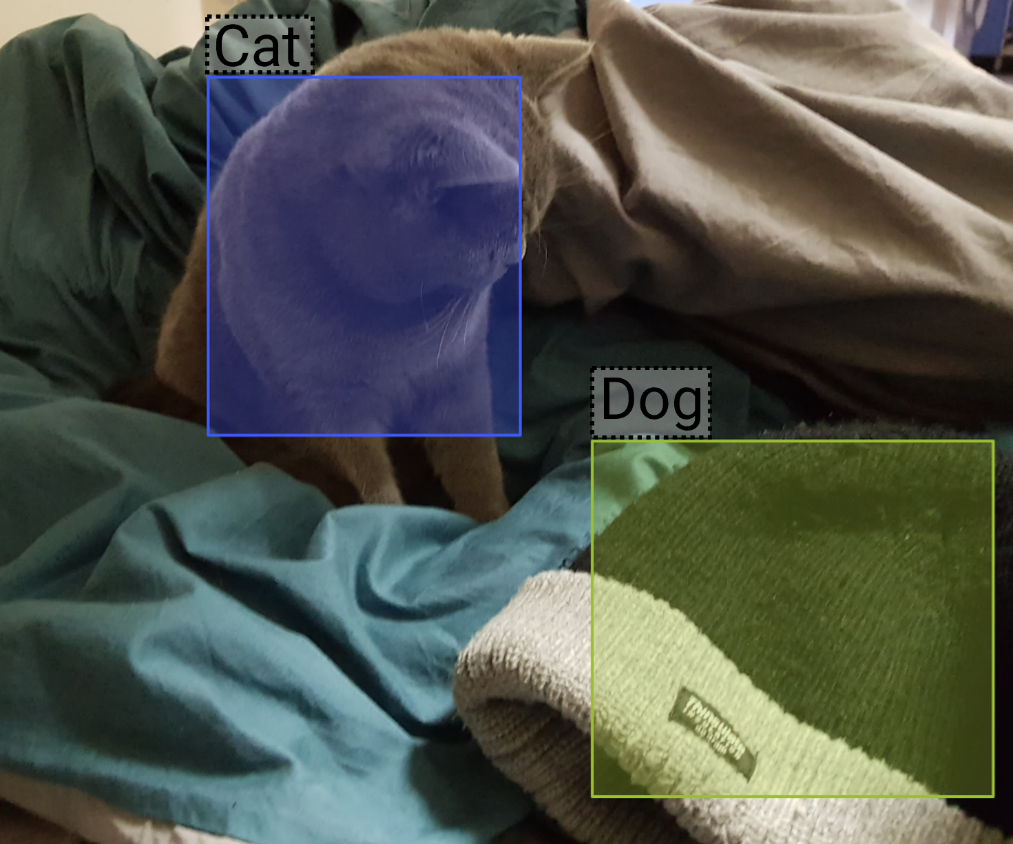
Example Object Detection Prediction (Click image to enlarge)
Ideally, predicted bounding boxes should have a high overlap with their associated ground truth bounding box. This will lead to a low localization loss.
Localization loss should reduce on the train set (the orange line) as training progresses.
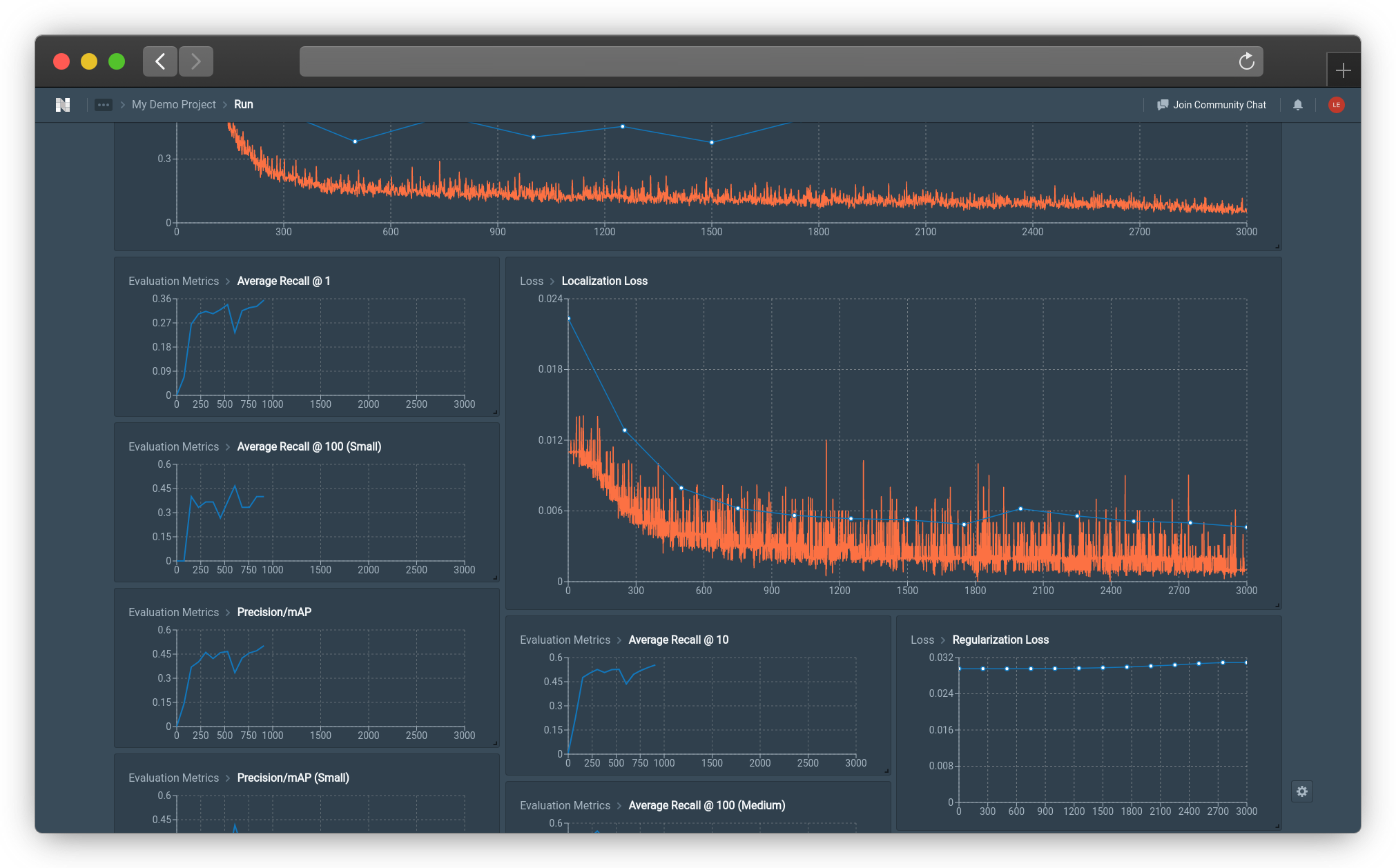
Localization Loss of Model (Click image to enlarge)
Regularization Loss
In Machine Learning models, regularization penalizes the weights of model coefficients, by adding an additional penalty term in the error function, proportional to the size of these penalized coefficients. This shrinks the penalized weights towards 0.
For neural network-based models, the weights of the connections between neurons can be penalized, leading to several benefits, including reducing overfitting.
Regularization Loss of Model (Click image to enlarge)
Detection Box Metrics
Comparing Detection Box Performance
Detection box metrics are all model agnostic. For a dataset with the same split for training set and evaluation set, these metrics can be compared across different models, regardless of the parent algorithm, model type, or image size.
Average Precision and Recall
We provide 6 metrics related to Average Precision, and 6 metrics related to Recall.
These 12 metrics are the same evaluation metrics used in the COCO object detection task, which is an annual object detection challenge on the COCO dataset.
Amongst the detection box metrics, Precision/mAP is calculated in a robust manner, and is generally a good metric to use in evaluating model performance. It is also the metric used in the COCO object detection task to rank models.
Mask Metrics
Mask metrics apply only to Mask RCNN models.
To understand these mask metrics, we briefly look at how Mask RCNN models work:
- Given an image, a Region Proposal Network (RPN) generates potential bounding boxes for objects (independent of object class)
- The bounding boxes predicted as being most likely to contain objects are selected
- The model splits into 2 parts here. For each bounding box,
3.1. the first part predicts the object in the bounding box, and further refines the bounding box coordinates around that object
3.2. the second part predicts, for each possible object class in the bounding box, whether each pixel is part of that object. An example is given below

Bounding Box Prediction (Left) v.s. Segmentation (Right) (Click image to enlarge)
There are 3 mask metrics used to measure loss — Mask Loss, Mask RPN Localization Loss, Mask RPN Objectness Loss.
Mask Loss
For each proposed region (from RPN) that contains an object, the ground-truth pixels for that object are compared with the predicted pixels for that object by the model. For example, if the proposed region contains a pen, the ground-truth pixels containing the pen are compared with the model's predictions for pixels containing a pen.
The higher the overlap between the ground-truth pixels and predicted pixels, the lower the mask loss.
Mask RPN Localization Loss
In Step 1 mentioned above, the top bounding boxes generated by the RPN are selected.
Some of these selected bounding boxes will indeed contain an object. The RPN Localization Loss measures how closely the selected bounding boxes match the ground-truth bounding boxes of the objects contained in the selected bounding boxes.
The higher the overlap between the ground-truth bounding boxes and predicted bounding boxes, the lower the
Mask RPN Objectness Loss
In Step 1 mentioned above, the top bounding boxes generated by the RPN are selected.
For each bounding box, the RPN also predicts a probability that the bounding box contains an object (independent of object class). The Mask RPN Objectness Loss measures how accurate these predictions are.
In an ideal scenario with low Mask RPN Objectness Loss, bounding boxes with a high predicted probability of containing an object will indeed contain an object, and vice-versa.
👋 Need help? Contact us via website or email
🚀 Join our Slack Community
💻 For more resources: Blog | GitHub | Tutorial Page
🛠️ Need Technical Assistance? Connect with Datature Experts or chat with us via the chat button below 👇
Semantic Segmentation Metrics
Semantic segmentation models classify every pixel in an image into a predefined class, without distinguishing between individual object instances. Unlike object detection which operates on bounding boxes, or instance segmentation which operates on per-instance masks, semantic segmentation produces a dense pixel-level prediction map where each pixel is assigned exactly one class label.
The key difference from Mask RCNN (instance segmentation) is that semantic segmentation does not separate individual object instances. For example, if two cars are side by side, instance segmentation will produce two separate masks — one for each car. Semantic segmentation will produce a single "car" region covering both vehicles.
Metrics used to measure semantic segmentation model performance can be categorized as:
| Type of Metric | Description |
|---|---|
Semantic Segmentation Loss Metrics | Measures how far the predicted pixel-level class map deviates from the ground truth during training |
Semantic Segmentation Evaluation Metrics | Measures the quality of the final predicted segmentation map against the ground truth |
Semantic Segmentation Loss Metrics
There are 3 loss metrics used to measure semantic segmentation performance during training: Focal Loss, Cross-Entropy Loss, Dice Loss.
Focal Loss
Cross-entropy loss (explained below) treats all pixels equally during training. In many real-world scenarios, certain classes occupy a much larger portion of the image than others — for example, "background" pixels may vastly outnumber "defect" pixels in an industrial inspection dataset. This class imbalance causes the model to become biased towards predicting the dominant class, since doing so already achieves a low cross-entropy loss.
Focal loss addresses this by down-weighting the loss contribution from pixels that the model already classifies correctly with high confidence, and up-weighting the loss from hard-to-classify pixels. This forces the model to focus its learning on the minority classes and difficult boundary regions that it struggles with.
In practice, focal loss is especially useful for datasets where the classes of interest are small or rare compared to the background. If focal loss is decreasing during training, it indicates that the model is improving at detecting these underrepresented classes.
If your dataset has a relatively balanced distribution of classes across the image, cross-entropy loss may be sufficient. Focal loss provides the most benefit when there is a significant class imbalance.
Cross-Entropy Loss
Cross-entropy loss is the standard loss function for classification tasks, applied here at the pixel level. For each pixel, the model outputs a probability distribution over all possible classes. Cross-entropy loss measures how different this predicted probability distribution is from the ground truth (where the correct class has a probability of 1 and all other classes have a probability of 0).
The loss is computed independently for each pixel and then averaged across all pixels in the image. A low cross-entropy loss means that for most pixels, the model assigns a high probability to the correct class.
Cross-entropy loss should decrease on the train set as training progresses. If the train loss decreases but the test loss begins to increase, this may indicate overfitting.
Dice Loss
Dice loss is derived from the Dice coefficient, which measures the overlap between two sets. In the context of semantic segmentation, it measures the overlap between the predicted segmentation mask and the ground truth mask for each class.
Unlike cross-entropy loss, which evaluates each pixel independently, dice loss considers the prediction holistically across the entire mask for each class. This makes it particularly effective for segmentation tasks because it directly optimizes for the spatial overlap that segmentation metrics (like IoU) care about.
Dice loss is computed per-class and then averaged across all classes. A dice loss of 0 indicates perfect overlap between predicted and ground truth masks, while a dice loss of 1 indicates no overlap at all.
It is common practice to combine dice loss with cross-entropy loss during training. Cross-entropy provides strong per-pixel gradients that help the model learn quickly in early training, while dice loss ensures the model optimizes for overall mask quality and is not dominated by the background class.
Semantic Segmentation Evaluation Metrics
There are 5 evaluation metrics used to measure semantic segmentation model quality: Average Precision (AP), Average Recall (AR), IoU Score, Pixel Accuracy, F1 Score.
Comparing Semantic Segmentation Performance
Semantic segmentation evaluation metrics are model-agnostic. For a dataset with the same split for training set and evaluation set, these metrics can be compared across different models, regardless of model architecture or image size.
Average Precision (AP)
Average Precision measures how well the model identifies pixels belonging to each class while avoiding false positives. For each class, precision is calculated as the proportion of predicted pixels for that class which are actually correct. AP then summarizes this across multiple confidence thresholds.
A high AP indicates that when the model predicts a pixel belongs to a particular class, it is usually correct. AP is typically reported as the mean across all classes (mAP).
Average Recall (AR)
Average Recall measures how well the model captures all pixels that truly belong to each class. For each class, recall is calculated as the proportion of ground truth pixels for that class which were correctly predicted by the model. AR summarizes this across multiple confidence thresholds.
A high AR indicates that the model successfully identifies most of the pixels belonging to each class, with few missed regions. AR is typically reported as the mean across all classes.
AP and AR represent a trade-off. A model can achieve high recall by aggressively predicting a class (at the cost of more false positives, lowering precision), or high precision by only predicting when very confident (at the cost of missing some true pixels, lowering recall). A good model achieves a balance between both.
IoU Score
Intersection over Union (IoU), also known as the Jaccard Index, is the most widely used metric for evaluating semantic segmentation. For each class, IoU is calculated as the area of overlap between the predicted mask and the ground truth mask, divided by the area of their union.
An IoU of 1.0 means the predicted and ground truth masks are identical for that class. An IoU of 0.0 means there is no overlap at all. The metric is typically reported as the mean IoU (mIoU) averaged across all classes.
IoU is considered a more informative metric than pixel accuracy because it penalizes both false positives and false negatives equally, and is not biased by class imbalance. For this reason, mIoU is the standard benchmark metric used in most semantic segmentation challenges and leaderboards.
Pixel Accuracy
Pixel accuracy is the simplest segmentation metric. It measures the percentage of pixels in the image that are correctly classified, calculated as the total number of correctly predicted pixels divided by the total number of pixels.
While intuitive, pixel accuracy can be misleading when there is a significant class imbalance. For example, if 95% of the image is background, a model that predicts everything as background will achieve 95% pixel accuracy despite failing to detect any objects of interest.
Pixel accuracy should not be used as the sole metric for evaluating semantic segmentation models. Always consider it alongside IoU score or F1 score, which provide a more balanced assessment of model performance across all classes.
F1 Score
The F1 score is the harmonic mean of precision and recall, calculated at the pixel level for each class. It provides a single metric that balances both false positives (pixels incorrectly assigned to a class) and false negatives (pixels that should belong to a class but were missed).
The F1 score ranges from 0 to 1, where 1 indicates perfect precision and recall. It is typically reported as the mean F1 score (macro F1) averaged across all classes.
The F1 score is particularly useful when you need a single number that captures both how complete and how accurate the model's predictions are for each class, without being dominated by class imbalance the way pixel accuracy can be.
Updated about 2 months ago